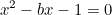
Consider a quadratic equation:
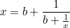
If we divide by x, this can be rewritten as:

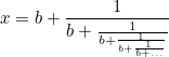
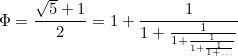
If we substitute the expression for x into the right hand side of the equation:
Repeating this infinitely, we arrive at a continued fraction.
In general, a continued fraction is an expression of the form

If bi = 1 for all i, like in the example given above, then the expression is called a simple continued fraction.
To avoid the cumbersome notation, simple continued fractions are written in the following form: ![\begin{equation} [ a_0;a_1,a_2,a_{3},\ldots , a_ n,\ldots ] \label{Ca} \end{equation}](https://plus.maths.org/MI/db21d27191a47a5e6fded63a5fe79b81/images/img-0013.png) .
.
Origins
Continued fractions were first used by Indian mathematician Aryabhata in the 6th century who used them to solve linear equations. In the 15th and 16th centuries, they re-emerged in Europe and Fibonacci attempted to define them in a general way. The term ‘continued fraction’ was first used by John Wallis in 1653 who, along with William Brouncker, studied their properties. Around the same period, Christiaan Huygens, a Dutch mathematical scientist, used continued fractions to build scientific instruments, finding a practical use for them. Finally, in the 18th and 19th centuries, Gauss and Euler explored their properties further.
Representing Numbers
Continued fractions can be both finite and infinite in length. If a continued fraction is finite, then each level can be evaluated (starting at the bottom), and hence will reduce to a rational fraction. However, if the continued fraction is infinite, it will represent irrational numbers. Examples of representations of irrational numbers as continued fractions are:
![\begin{equation} e=[2;1,2,1,1,4,1,1,6,1,1,8,1,1,10,\ldots ] \label{C1} \end{equation}](https://plus.maths.org/MI/1d0dab7b8098f4122bd17b2bff882528/images/img-0008.png)
![\begin{equation} \sqrt {2}=[1;2,2,2,2,2,2,2,2,2,2,2,2,2,2,2,\ldots ] \label{C2} \end{equation}](https://plus.maths.org/MI/1d0dab7b8098f4122bd17b2bff882528/images/img-0009.png)
![\begin{equation} \sqrt {3}=[1;1,2,1,2,1,2,1,2,1,2,1,2,1,2,\ldots ] \label{C3} \end{equation}](https://plus.maths.org/MI/1d0dab7b8098f4122bd17b2bff882528/images/img-0010.png)
![\begin{equation} \pi =[3;7,15,1,292,1,1,1,2,1,3,1,14,2,1,1,2,2,2,2,1,84,2,\ldots ] \label{C4} \end{equation}](https://plus.maths.org/MI/1d0dab7b8098f4122bd17b2bff882528/images/img-0011.png)
It can be seen that all expansions, except for  have simple patterns. Therefore, continued fractions can reveal hidden patterns about seemingly random numbers.
The expression of real numbers as continued fractions can be said to be the most “mathematically natural” representation, compared to decimal representation, due to several desirable properties:
- The continued fractions representation for a rational number is finite, whereas the decimal representation of a rational number can be finite or infinite with a repeating cycle.
- Every rational and irrational number has a unique continued fraction representation.
- The real numbers whose continued fraction eventually repeats are the quadratic irrationals (an irrational number that is the solution to some quadratic equation with rational coefficients). For example, in the quadratic equation that I demonstrated above, which led to a continued fraction, if we say b=1, this would lead to the golden ratio.
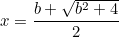
so
- The approximations produced in finding the continued fraction representation of a number, by truncating the continued fraction, are the ‘best possible’.
Expanding on the last point, we can approximate an irrational number using a rational fraction which is obtained by ‘chopping off’ the continued fraction expression at order n – the convergents of the continued fraction. As n increases, the difference between the irrational x and its convergent decreases:

Hope you enjoyed this post!

How can we calculate continued fraction for Pi?
LikeLike
To calculate the convergents of π, set a0 = ⌊π⌋ = 3, define u1 = 1/π − 3 ≈ 7.0625 and a1 = ⌊u1⌋ = 7.
Then u2 = 1 / u1 − 7 ≈ 15.9966 so a2 = ⌊u2⌋ = 15,
Continuing like this, you can determine the infinite continued fraction of π as [3;7,15,1,292,1,1..]
LikeLike
But how do I know the value of pi? How do I know it’s infinite (equivalent to saying that pi is irrational number)? If I already know the value of pi to certain decimal places why I would be interested to find it’s best rational approximation to some fraction upto same number of decimal places?
LikeLike
My best answer to this question is that continued fractions help us find fractions that approximate this irrational number, (such as 22/7 for pi) by using the convergents of the continued fraction expression. This article explains this is more detail: http://blogs.scientificamerican.com/roots-of-unity/what-8217-s-so-great-about-continued-fractions/
LikeLike
See, I am a bit sentimental about continued fractions (see my comments here: http://wp.me/p1RYhY-XB).
I ask such questions to people interested in continued fractions, so as to motivate them to dive deeper. Here are the answers:
(1) We know the value of pi from infinite series (eg: https://en.wikipedia.org/wiki/Leibniz_formula_for_%CF%80). [Proving n th root of a number to be a rational/irrational is child’s play!]
(2) Pi was proved to be irrational for the first time using continued fractions (https://en.wikipedia.org/wiki/Proof_that_%CF%80_is_irrational).
(3) Even if I know the value of pi to certain decimal values, my rest of the values (000000…) are no where close to original value. But the fraction I get from “truncated” continued fraction is “best possible” representation of pi with respect to remaining decimal values (which I haven’t even calculated!!).
I would suggest you to ask and answer similar questions for Euler constant (e).
LikeLiked by 1 person