A space-filling curve is a curve whose range covers the whole 2D unit square. We generally imagine space-filling curves as an infinite version of a finite construction using an iterative process.
Peano Curve
The first such curve was first discovered by Guiseppe Peano in 1890, and is thus given the name the ‘Peano Curve’. Peano’s Curve is a surjective, continuous function from the unit interval onto a unit square. However, it is not injective (a one-to-one function that preserves distinctiveness).
Peano’s curve may be constructed using a sequence of steps. In step i, each square s of Si − 1 is partitioned into nine smaller equal squares, and its centre point c is replaced by a contiguous subsequence of the centres of the nine smaller squares. This subsequence is formed the following way:
- Group the nine smaller squares into 3 columns
- Order the centres contiguously within each column
- Order the columns from one side of the square to the other so that the distance between each consecutive pair of points in the subsequence equals the side length of the small squares.
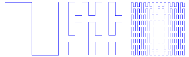
The Peano curve itself is the limit of the curves as i goes to infinity.
Hilbert Curve

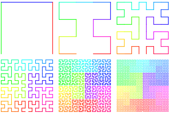
In 1891, Hilbert published a variation of Peano’s construction. Hilbert was the first to use a picture, which was included in the article, to help visualise the construction technique.
The difference between the Peano and Hilbert curve is that the latter is based on subdividing squares into four equal smaller squares instead of into nine equal smaller squares. Hence, Hilbert maps intervals of length 2-2n into squares of size 2-n×2-n, whereas Peano’s construction is equivalent to mapping intervals of length 3-2n into squares of size 3-n×3-n.
Other Space Filling Curves
Moore Curve
The Moore Curve could be thought of as the union of four copies of the Hilbert curves combined in such a way to make the endpoints coincide.
Wunderlich Curve

Read this article for more details on its construction.
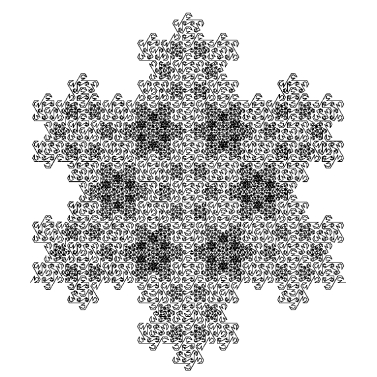
Koch Snowflake
In my opinion, space-filling curves are another example of how mathematics can be beautiful – creating wonderful shapes and images.
Let me know what you think! M x

Cool variant of Hilbert Curve: https://mathlesstraveled.com/2016/02/07/post-without-words-5-explained/
LikeLike
Going bananas with Hilbert, R code for generating Space-filling curves: https://aschinchon.wordpress.com/2016/02/01/going-bananas-with-hilbert/
LikeLiked by 1 person
Wow, so cool! Thanks for sharing..
LikeLike
I was actually thinking about space filling curves recently so this came at a very good time! I started wondering why we couldn’t just use a kind of “up and down” curve that started at (0,0), went up to (0,1), along for a bit then down again. The iterations would be achieved by compressing this shape width-ways by half, and then adding on a copy. Presumably if this was a space filling curve, it would be explained somewhere as the simplest example so it probably isn’t the case…
/var/folders/80/_z39_pdd7v31gnvrj8xb0c880000gn/T/com.apple.iChat/Messages/Transfers/IMG_3140.JPG
I think this is how it goes wrong. Joining iterations together wouldn’t work without a “sticking out bit”. e.g. Go up from (0,0), to (0,1), along to (0.99,1), back down to (0.99,0), then along to (1,0). As with all of the horizontal sections, the lengths would get arbitrarily small while the vertical lines would get arbitrarily closer, seeming to fill the space. However at any iteration, a neighbourhood of (1,1) would not see any of the curve.
Do you agree? Is this the only way this example fails?
LikeLike
That image didn’t work
LikeLike
I think your idea is similar to a snake curve, shown in the video I posted below (https://www.youtube.com/watch?v=DuiryHHTrjU). I do think your reasoning is correct in how your variation would fail, but I do think there is a way to make it work as a space-filling curve, as explained in the video.
LikeLike
Ah true, it does seem to work. I forgot you could join segments together with extra lines, so my argument doesn’t work. It’s just not got all the same nice properties as one of the other space filling curves. Thanks 🙂
LikeLiked by 1 person
I had a go with the reflect and move method, not sure it is totally correct, but it appears to work. I used MS Paint. Here are the links:
LikeLiked by 1 person
The video I posted in a comment below explains the construction very clearly. Have a watch if you’re interested!
LikeLiked by 1 person
Excellent video, thanks. He was a bit sketchy on the Peano curve, but its the same idea as for the hilbert curve, with a factor of 3 rather than 2. This stuff came up some years ago, when high definition TV was still in the future. I think that the LCD approach rendered it unnecessary.
Did he play the lion music?
LikeLike
How did you insert picture in comments?
I could draw Hilbert curve by hand following this tutorial: https://bentrubewriter.com/2012/04/26/fractals-you-can-draw-the-hilbert-curve-or-what-the-labyrinth-really-looked-like/
LikeLiked by 1 person
I’ve always found this interesting, along with Cantor’s middle third set, and continuous curves that are nowhere differentiable.
I looked at the illustration of the first three iterations of the Peano curve and thought there was something wrong. The scale changes ! each diagram refers to a different square.
I followed your instructions, but they were too vague. I did the dots for step 2, joined them to get the second picture, and then spotted the symmetry. Each of the nine little squares is a reflection of each of the adjacent little squares. Just have to join them together. Now take the new picture (the second one) and do the same reflections, across and down, join them together in the now obvious way and get the third picture. This procedure just has to continue !!!!!
All that is needed now at each step is to shrink the new picture to the same square size as the previous.
I then went to wikipedia and read a bit more about Peano’s square. This procedure is buried in the article, in a very cryptic way.
LikeLike
Thank you for adding more detail! Sorry for not including all the specifics. Wikipedia has a lot of information, however I sometimes find that some of the maths on there is a bit inaccessible.
LikeLike
What lead to idea of Space Filling Curves? Why do we study them?
LikeLike
Peano was motivated by Cantor’s work on infinity (specifically his result that the “infinite number of points in a unit interval is the same cardinality as the infinite number of points in any finite-dimensional manifold”) to find a mapping from a one-dimensional line into two-dimensional space, in such a way that the line crosses every single point in that space.
Hence, Space-filling curves allows you reduce higher-dimensional proximity
problems (e.g. nearest neighbour search) to a one-dimensional problem.
I really recommend watching this video, it is really interesting: https://www.youtube.com/watch?v=DuiryHHTrjU
LikeLiked by 1 person
Nice! Never thought so deep.
I really enjoy 3Blue1Brown videos. This one is particularly wonderful. Comments on this video are really interesting, like:
(1) The function is actually not a bijection. Every point in the unit square has an infinite number of pre images.
(2) The function is not injective. It’s actually impossible to have in injective space filling curve.
(3) The cardinal numbers of 1D and 2D spaces are the same. Having the same cardinality just means there exists some bijection between the two, but this says there exists a continuous surjective map between the two.
(4) If Rudin explained analysis the way you do, I wouldn’t be so tempted to set his book on fire.
Thanks for sharing this post, I hope to learn more about it during my Topology course 🙂
LikeLiked by 1 person
Thank you for the summarizing the video comments. So glad you enjoyed the post!
LikeLiked by 1 person
I now have proof of the following two facts:
(1) there can’t be continuous bijective map between R and R^2
(2) Hilbert curve is a continuous surjective map from R to R^2.
Proofs are quite elementary, thanks to my Analysis professor. 🙂
LikeLike
Would you consider writing a blog post to share them?
LikeLiked by 1 person
Here are the proofs:
(1) You have to use connectedness property as well as the property that R^2 is complete. I found similar argument on Stackexchange: http://math.stackexchange.com/q/1092148/214604
(2) I typed the proof neatly, see: https://gaurish4math.files.wordpress.com/2016/04/spacefillingcurves.pdf
LikeLiked by 1 person
Sorry, there was a typo in (2) so I updated the file.
Updated File Link : https://gaurish4math.files.wordpress.com/2016/04/spacefillingcurve.pdf
LikeLike